The Extended Exponential Range Reduction Curve

With the increase in complexity in tonemapping and the emergence of full Image Formation Models (IFMs), it has become increasingly beneficial to treat the mathematical curve used to compress a scene-referred buffer as separate subject matter from tonemapping, as the ways to approach it are many. Hereafter, such curves will be referred to as Range Reduction Curves (RRCs) for the sake of clarity.

This article describes the construction of an RRC based on the exponential function. A more complete method of tonemapping was developed alongside it, but it is not fundamental to it, thus it will be delegated to a future blogpost.

It’s assumed that the reader has a degree of familiarity with the topic, so the basics are not covered here. Otherwise, you may find a good crash-course here.

1. Design Philosophy

After working with many curves over the years, a set of criteria started to emerge:

Modularity - If it is deemed necessary to bypass a part of the curve, it should be done easily.
Flexibility - Dynamic range may vary greatly and a candle-lit indoors scene is better suited to a vastly different curve in comparison to sunny mid-day conditions.
Visual completeness - Extensive post-processing must not be a requirement for a visually pleasing result to be achieved.

2. Constructing the Curve

This section will go over the design process. All image examples have had the RRC applied per-channel for the sake of brevity, though it’s not a method I endorse. The example image comes from Polyhaven.

The exponential curve is used as a starting point:

$$1-e^{-x}$$

Fig. 1

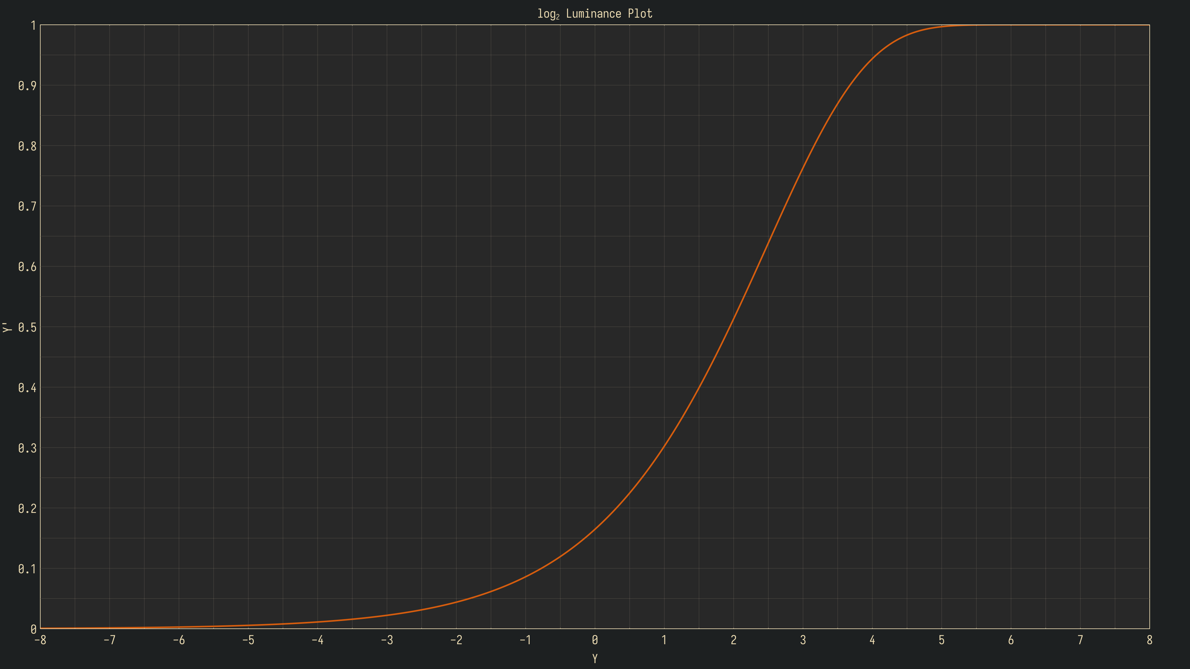
Here’s an example, the left half has had the linear input clamped and the right the exponential RRC applied.

Ex. 1

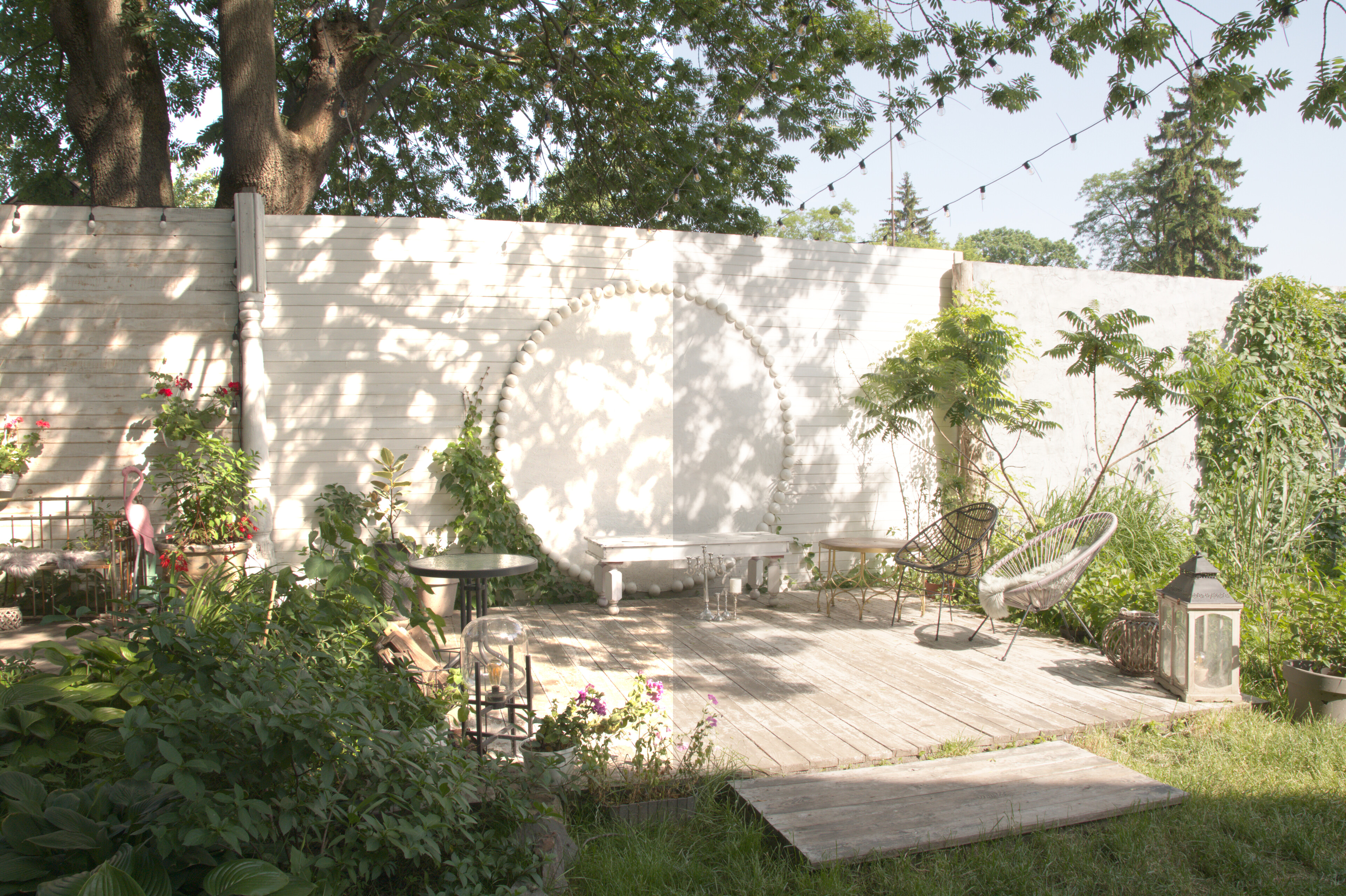
It’s a visually pleasing result but there’s a few evident issues:

Lack of contrast in the shadows
Lack of headroom, we’ve not even 5 stops of dynamic range above middle gray.

We shall address the highlights first. A simple way to control the shoulder of the curve is to apply it in a non-linear domain. Let’s introduce a parameter called r, for range:

$$\left(1-e^{-x^{\frac{1}{r}}}\right)^r$$

Fig. 2

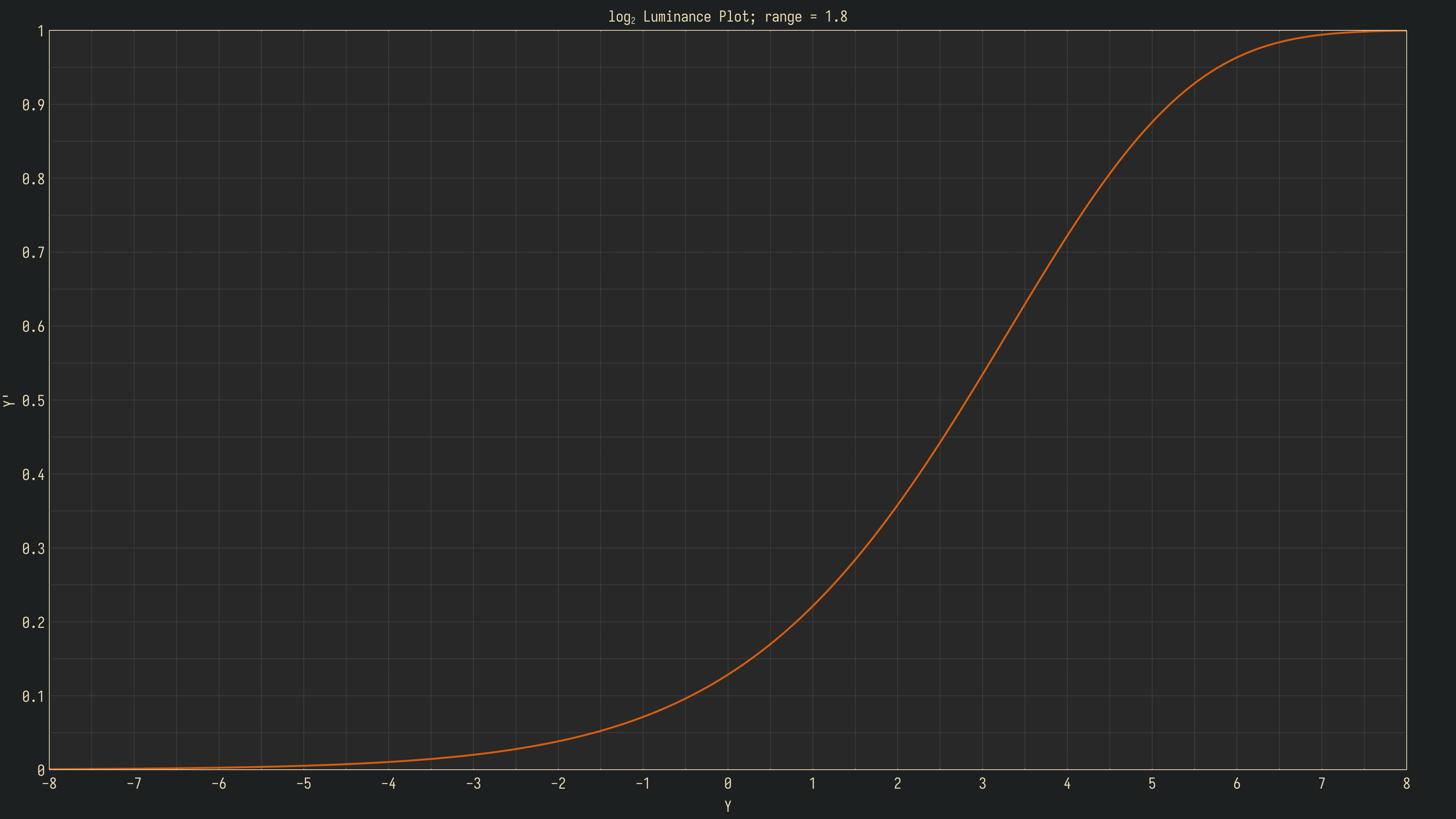
With r = 1.8, the headroom increases to over 7 stops, with the possibility to go much higher. r < 1 will reduce headroom, which may be of use for scenes with low DR.

Ex. 2

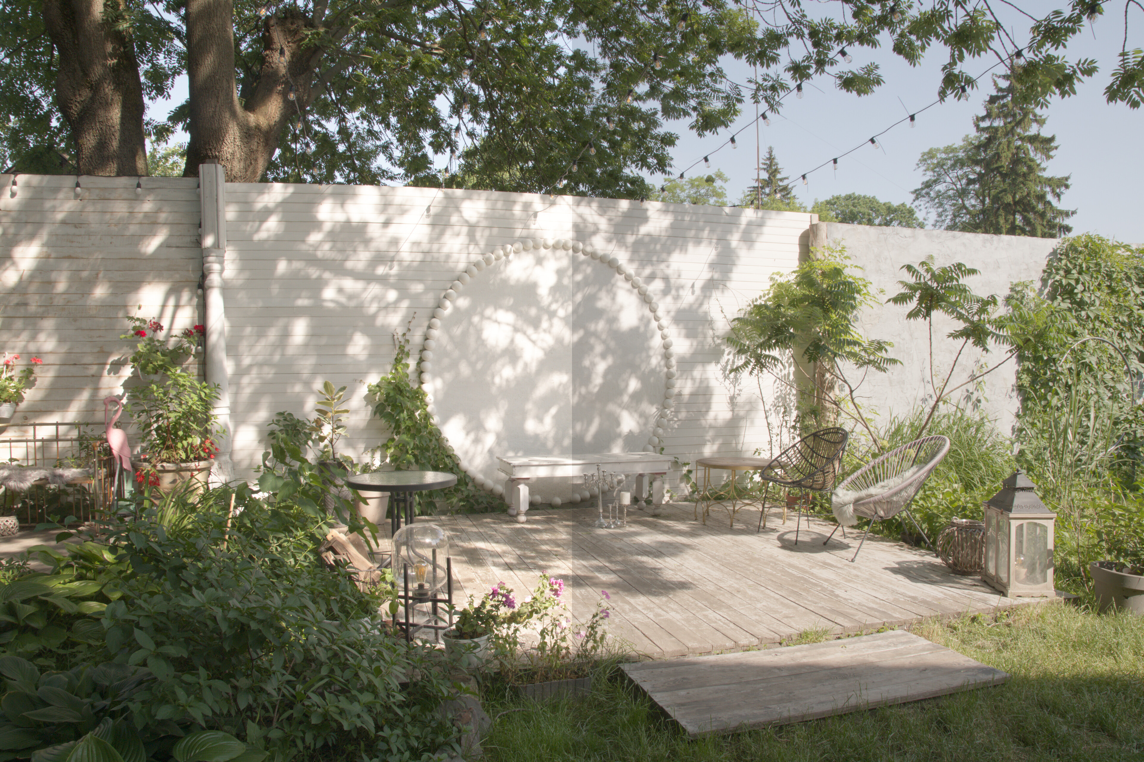
The increased highlight range allows the recovery of some of the texture on the walls that’s otherwise lost. As always such adjustments are a matter of taste. According to my own, a toe region is necessary.

One approach that fits the outlined design philosophy is to use a rational function, namely:

$$\frac{x^2}{x+t}$$

After integrating it into the curve, the result is this:

$$\left(1-e^{-{\left(\frac{x^2}{x+t}\right)}^{\frac{1}{r}}}\right)^r$$

Fig. 3

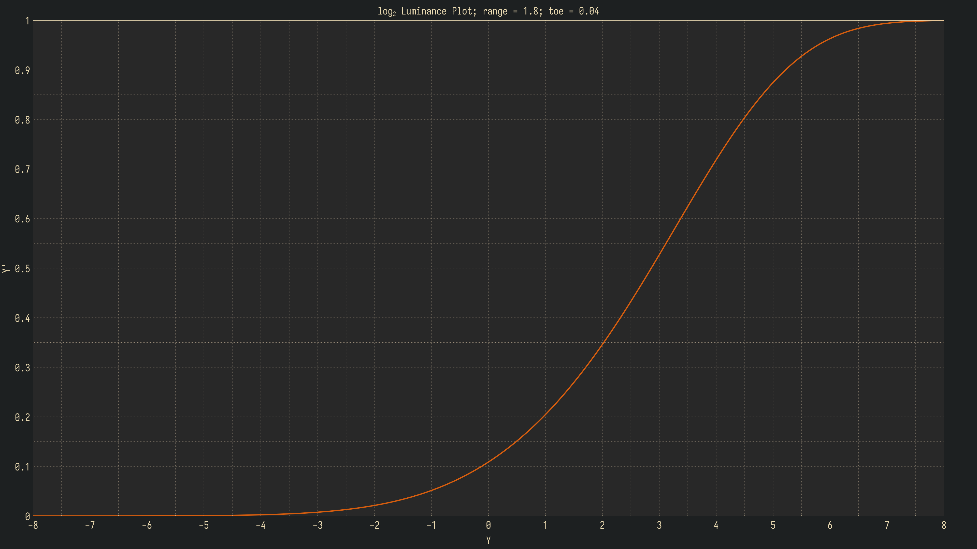
The order of operations is a matter of taste and some may find it preferable to compress the shadows after entering the non-linear domain, but this will tie the behaviour of the toe region to the shoulder region, which may be a drawback in terms of usability.

As established, on the left is the previous iteration and on the right, the newly made additions.

Ex. 3

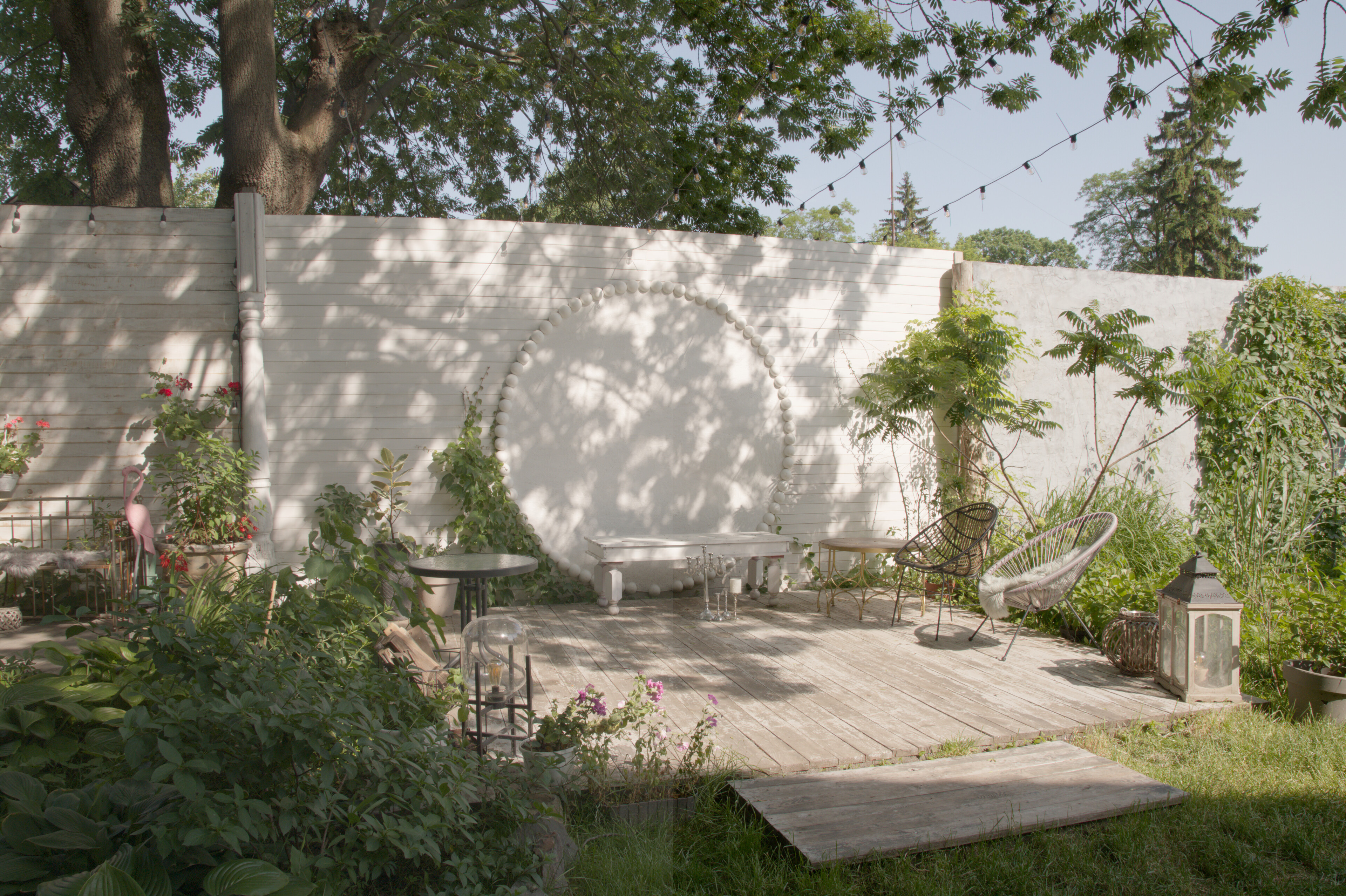
The change is much less dramatic this time around, but now there’s a lot more definition in the darker areas without a loss of detail.

At this point, a satisfactory result’s been achieved, but there’s still low-hanging fruit to be picked and 2 further additions will be made.

The informed reader may recall that a common addition to the exponential RRC is a simple exposure / gain bias:

$$1-e^{-xg}$$

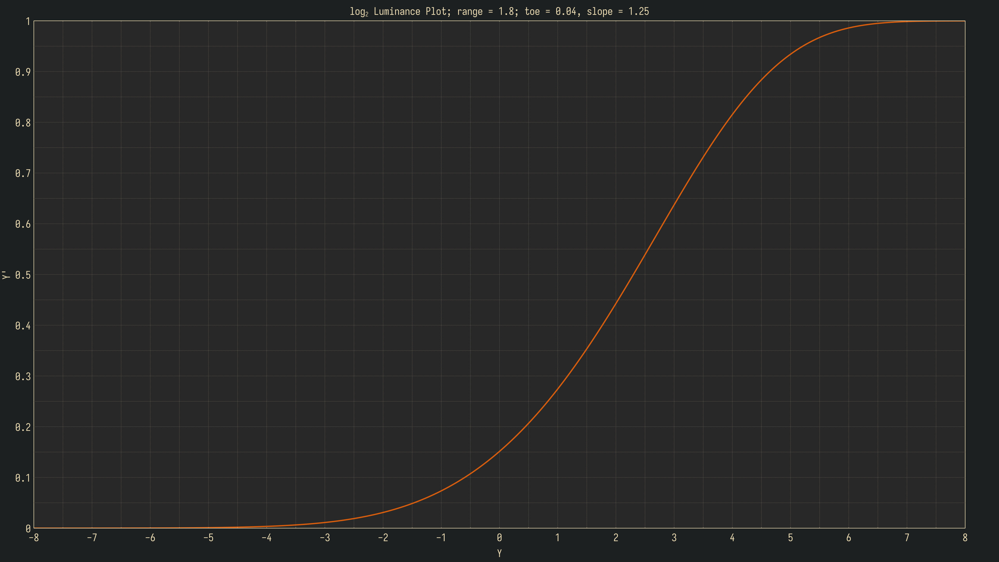
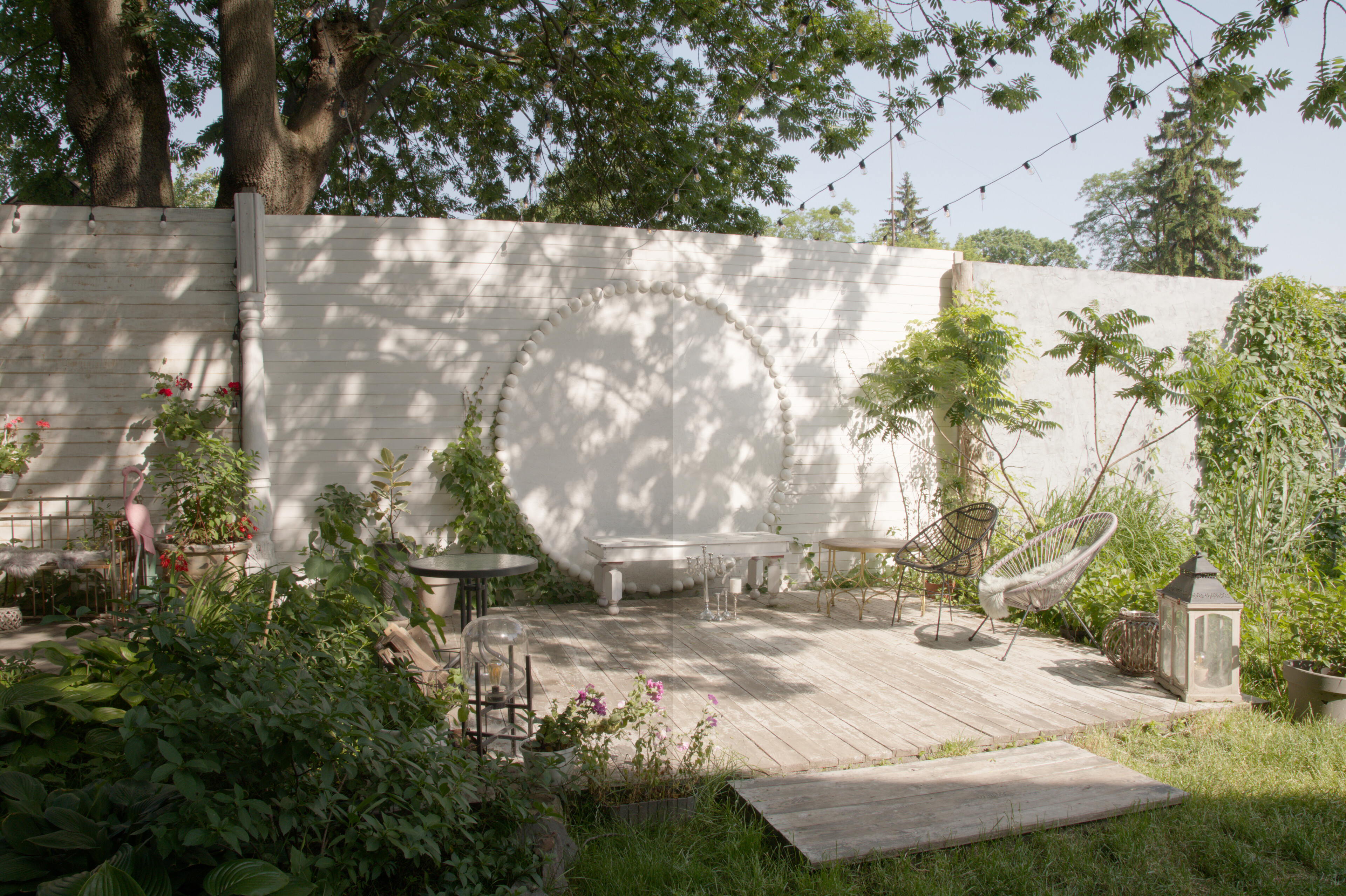
However, since this stage is performed in a non-linear, γ-warped domain, such a parameter will control the angle and length of the midtones section instead. Let’s introduce a new variable s, for slope:

$$\left(1-e^{-\left({\left(\frac{x^2}{x+t}\right)}^{\frac{1}{r}}\right)s}\right)^r$$

Fig. 4

Ex. 4

Last but not least, a common and simple approach of boosting or cutting contrast is via a power curve. This is quite beneficial for us, since it’s computationally free. Let us replace the numerator in the range section of our function with γ.

$$\left(1-e^{-\left({\left(\frac{x^2}{x+t}\right)}^{\frac{\gamma}{r}}\right)s}\right)^r$$

Fig. 5

Ex. 5

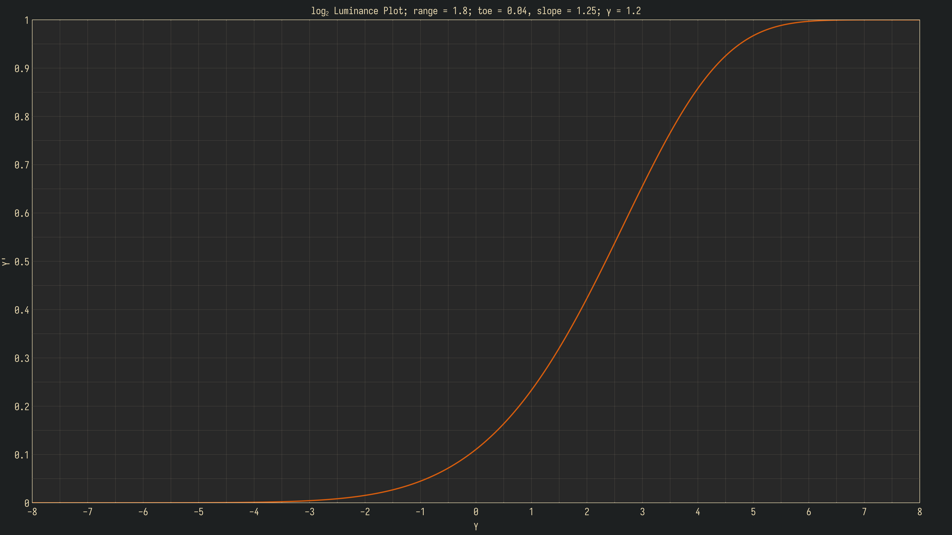
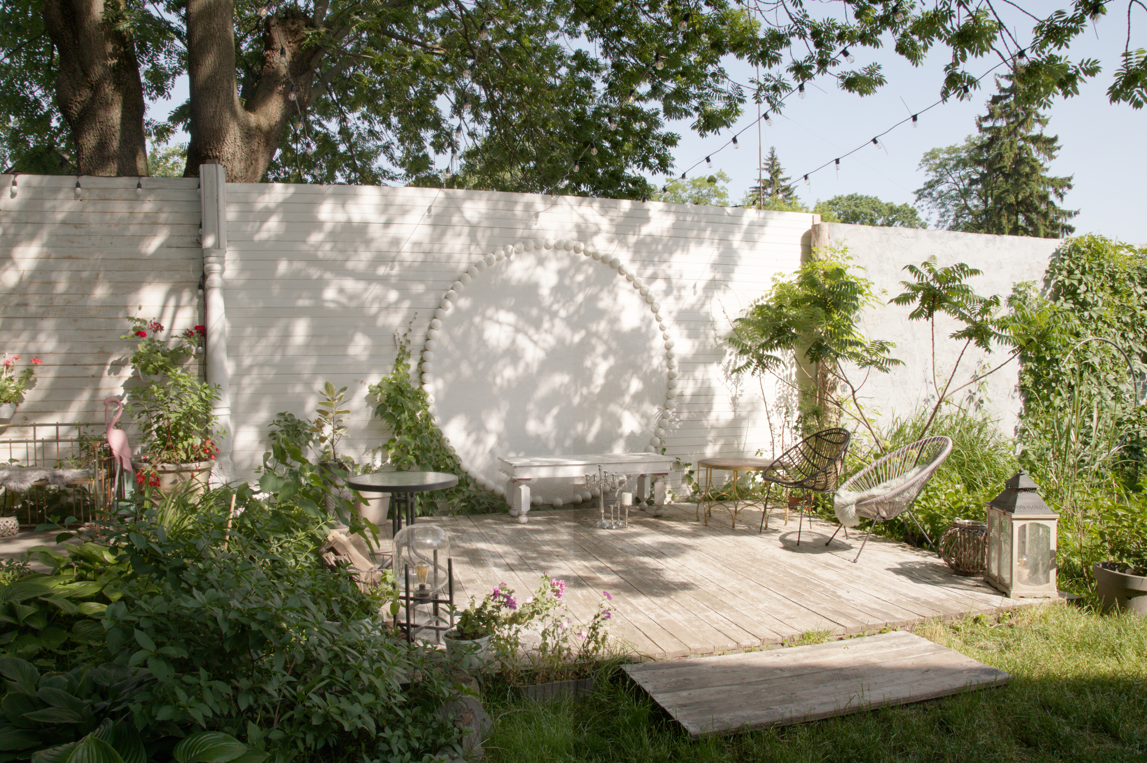
3. In practice

It is worth noting that in the examples the parameters used were quite modest and the curve can be pushed much further. Here’s a final example that’s been pushed a bit more, with a slight exposure re-adjustment.

Fig. 6

Ex. 6

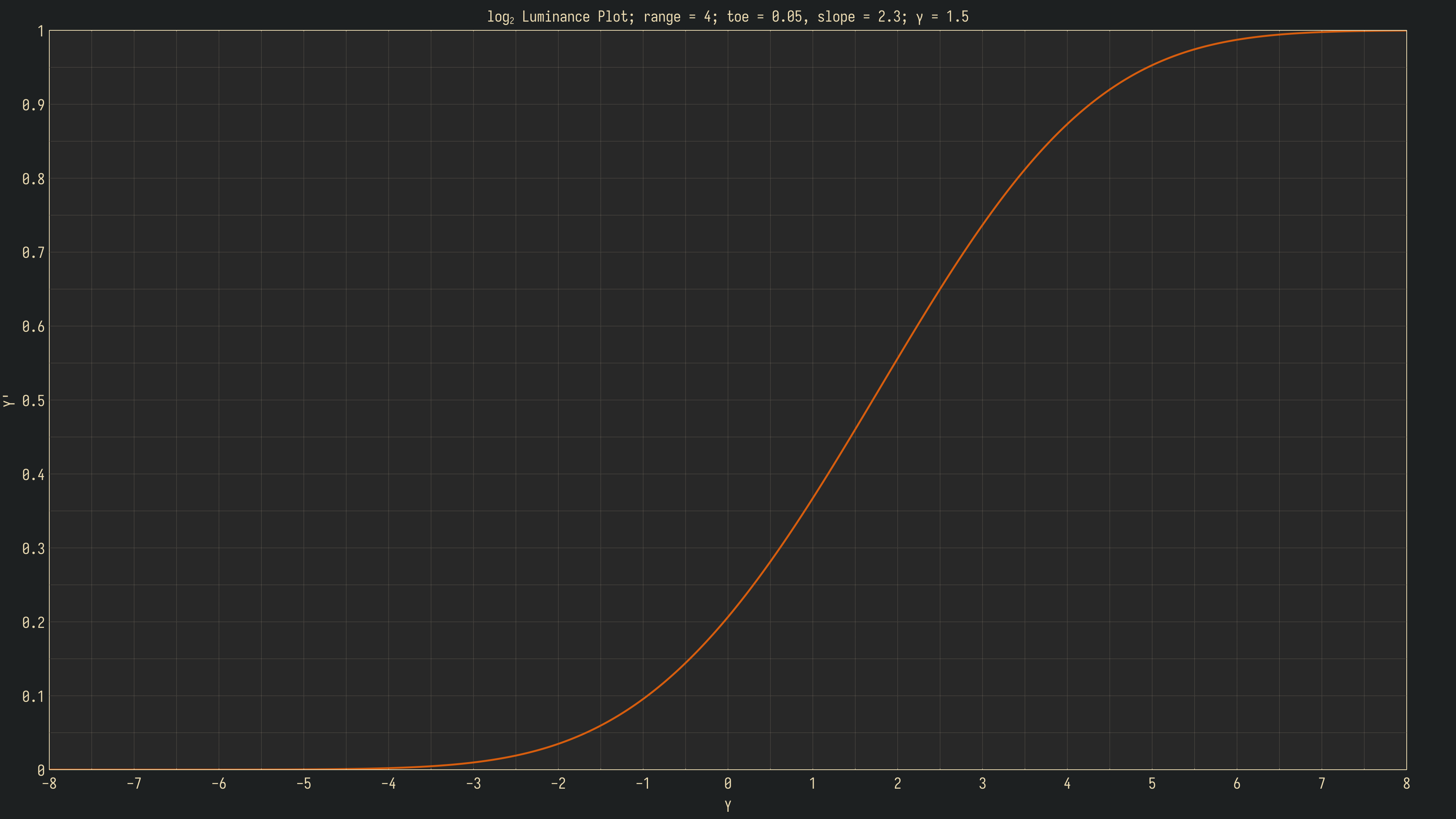
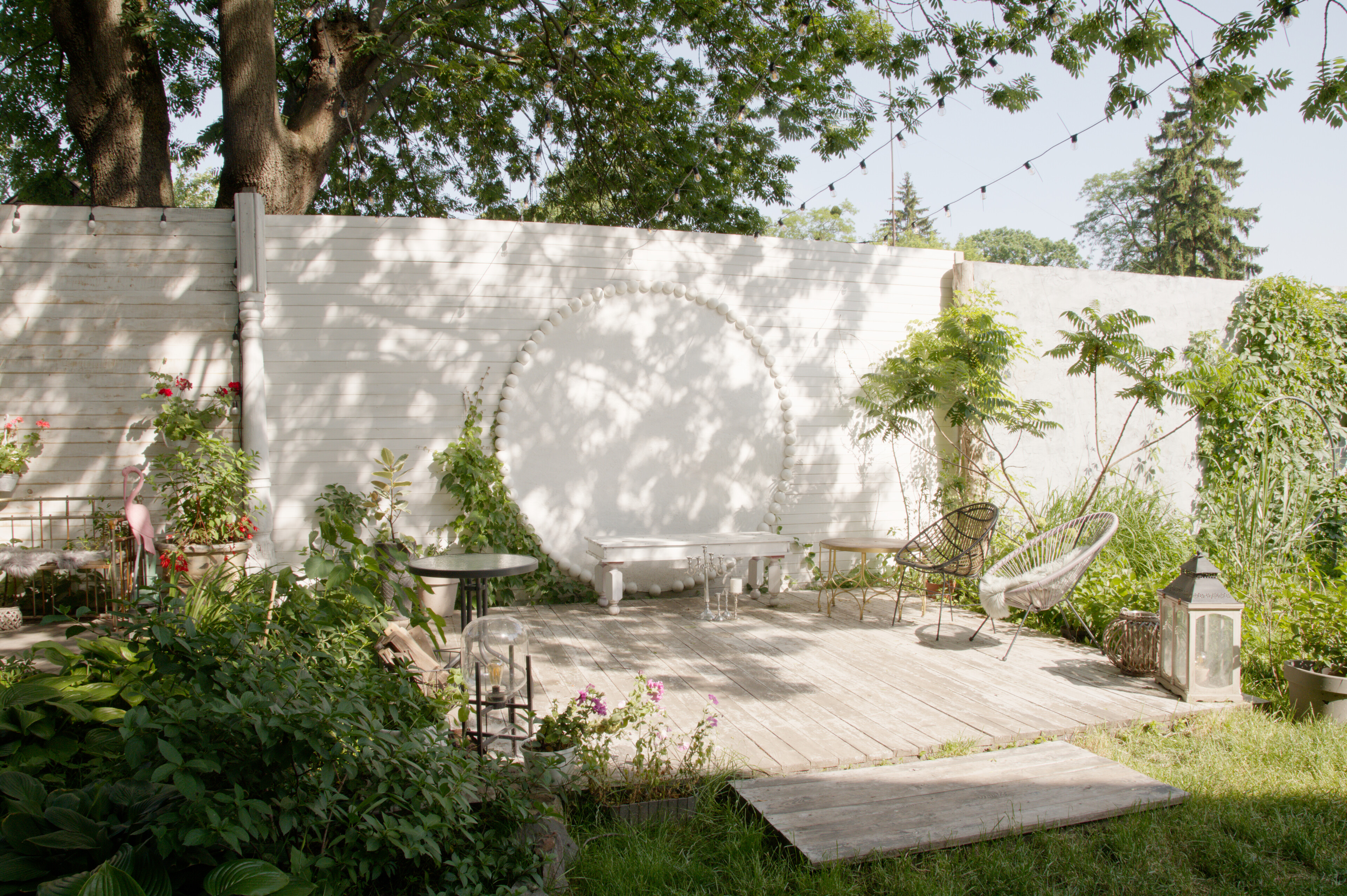
Finally, here’s a GLSL snippet:

float rrc_ee(float x,
	      float t,
	      float s,
	      float y,
	      float r)
{
	return pow(1.0 - exp(-pow((x * x) / (x + t), y / r) * s), r);
}